Correlation and Regression Projects

Objectives

The correlation and regression project is designed to:
(1.) Meet one of the learning objectives of the VCCS (Virginia Community College System) standards for:

(a.) MTH 155: Statistical Reasoning
(Presents elementary statistical methods and concepts including visual data presentation, descriptive statistics, probability, estimation, hypothesis testing, correlation and linear regression.).

(b.) MTH 245: Statistics I
(Presents an overview of statistics, including descriptive statistics, elementary probability, probability distributions, estimation, hypothesis testing, correlation, and linear regression.).

(2.) Draw a scatter diagram between two variables by technology.

(3.) Calculate the Pearson linear correlation coefficient between two variables by formulas.

(4.) Determine the Pearson linear correlation coefficient between two variables by technology.
The technology that we shall use are:
Texas Instruments (TI)-series calculator
Google Spreadsheets
Microsoft Excel

(5.) Calculate the linear regression equation between two linearly-correlated variables by formula.

(6.) Determine the least-squares regression line between two linearly-correlated variables by technology.
The technology that we shall use are:
Texas Instruments (TI)-series calculator
Google Spreadsheets
Microsoft Excel
Pearson Statcrunch

(7.) Meet the QM (Quality Matters) and USDOE (United States Department of Education) requirements for distance education as regards the provision of RSI (Regular and Substantive Interaction).
Federal Register: Distance Education and Innovation
St. John's University: New Federal Requirements for Distance Education: Regular and Substantive Interaction (RSI)
Student – Content Interaction: Very high
Student – Student Interaction: Flexible
Student – Faculty Interaction: Very High

Project Requirements

(1.) Data (Dataset): What dataset(s) should you use?
There are five approved ways to get the dataset(s).
Use any or combination of them.

(a.) Textbook (eBook) Datasets
You may use any of the applicable datasets from your eBook











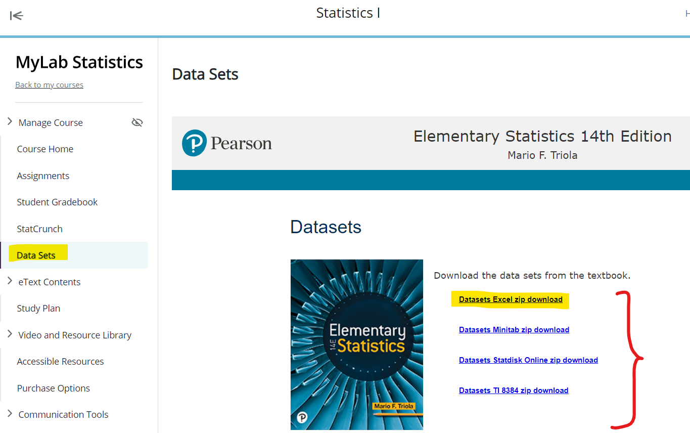
(b.) MyLab Math (MLM) Datasets
You may use any of the applicable datasets from your MLM assignments.

(c.) Datasets from the U.S Government website: United States Government's Open Data: Datasets
You may use any of the applicable open datasets from the U.S government.

(d.) RStudio Datasets:
You may use any of the applicable built-in datasets from RStudio.

(e.) Data Collection from my Students. (This option is for onsite (traditional/in-class) students only.)
Please see me in the Office during Student Engagement hours so we can discuss the data collection methods and other requirements.

Please Note:
(I.) Any other dataset besides the ones mentioned should be pre-approved by me.
(II.) If you cannot find any dataset, please contact me via my school email (not via the Canvas messaging system).

(2.) Type of Linear Relationship
The relationship between any two variables may be:
(a.) Positive Linear Correlation
(b.) Negative Linear Correlation
(c.) No Linear Correlation.
At least an application of any two types of linear relationship is required.
This implies that a minimum of two applications is required for the project.
Please review the Example Guides for all three types of linear relationships.
Each application should be a word problem.
The predictor variable and the response variable should be real-world applied concepts.

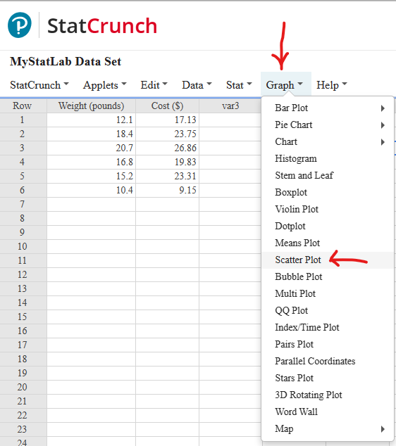
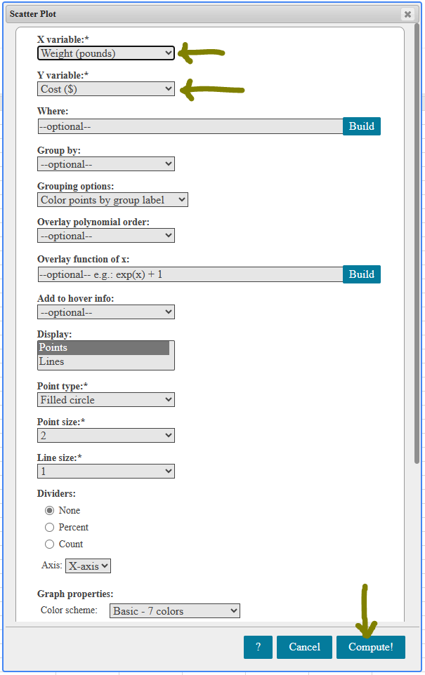
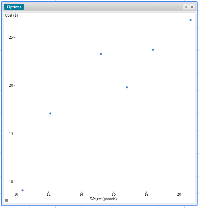
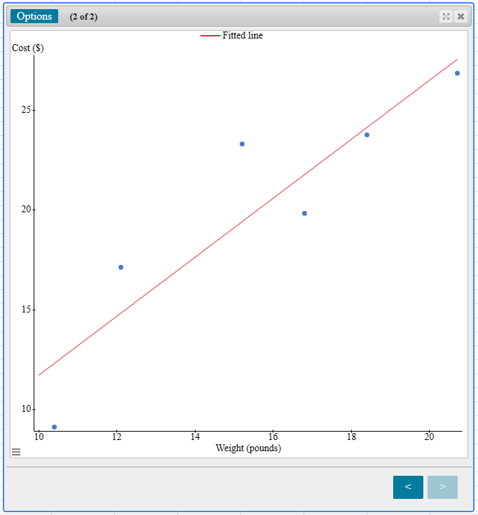
(3.) Scatter Diagram
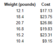
Using technology, draw a scatter diagram for each application.
Interpret the scatter diagram.

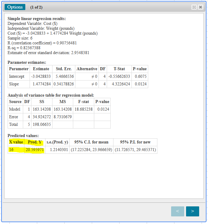
(4.) Linear Correlation Coefficient
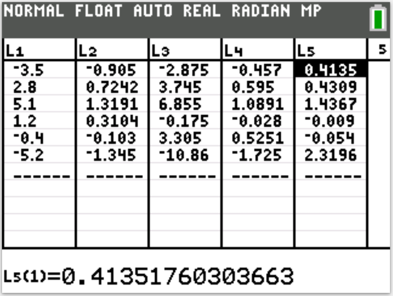
Calculate the linear correlation coefficient using formulas.
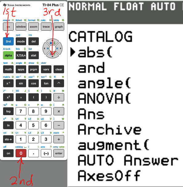
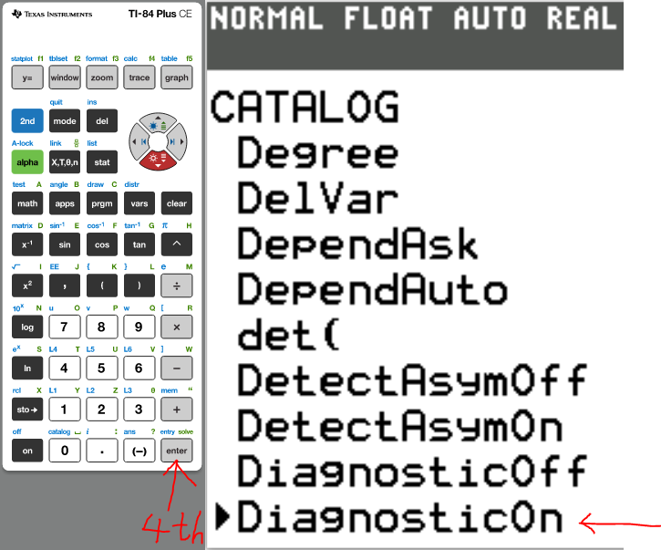
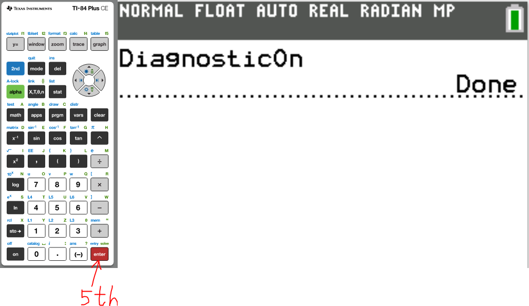
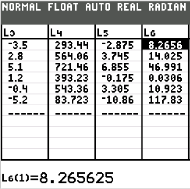
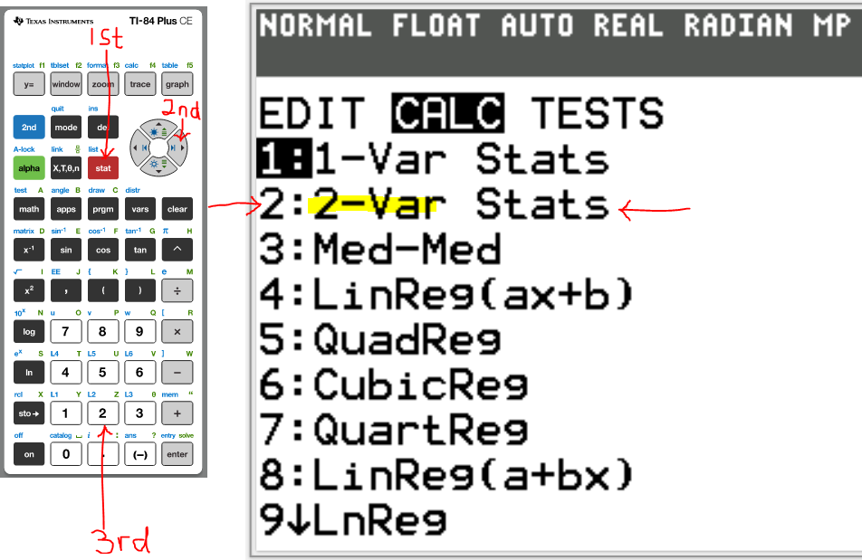
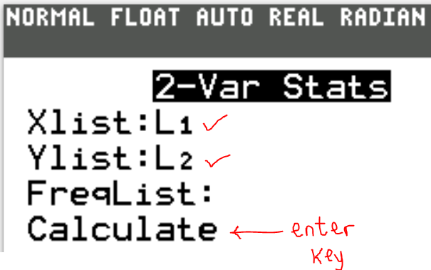
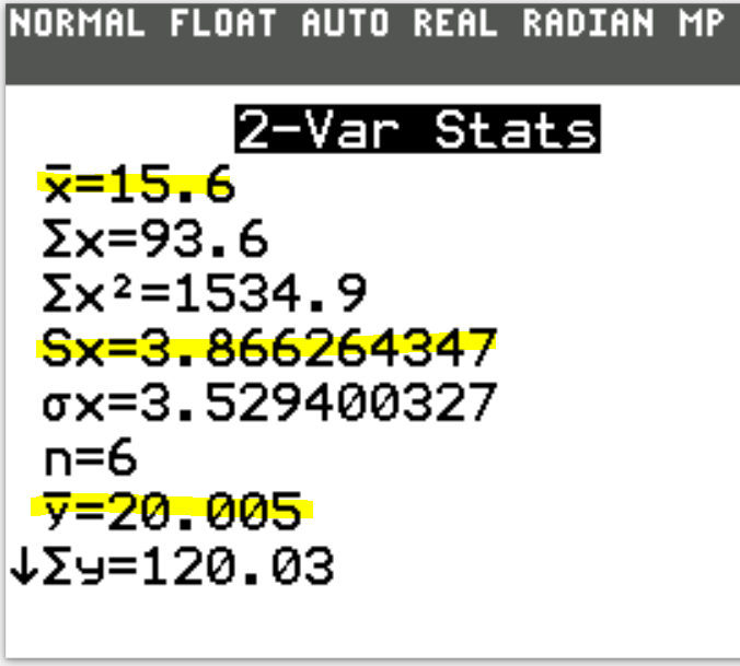
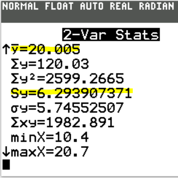
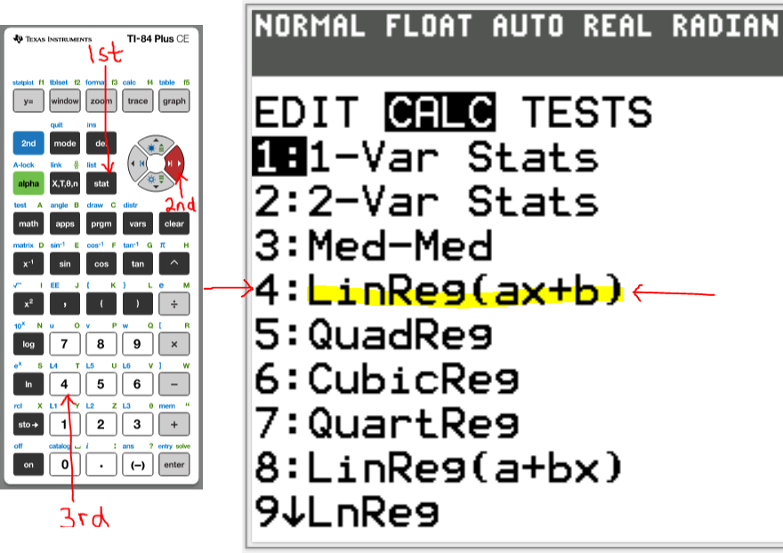
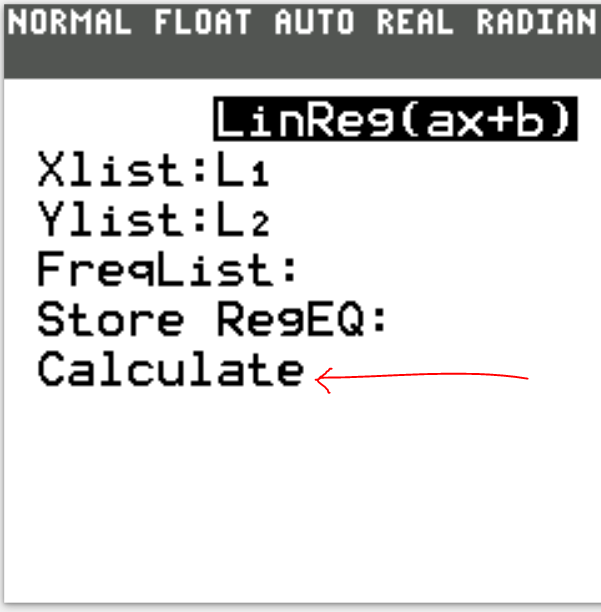
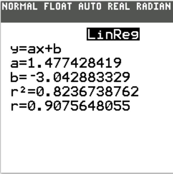
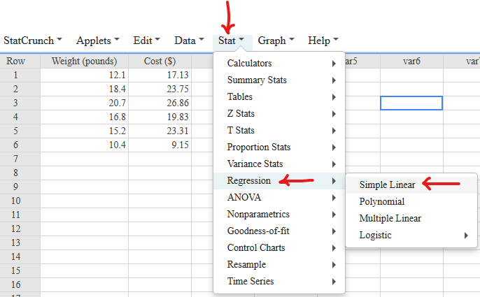
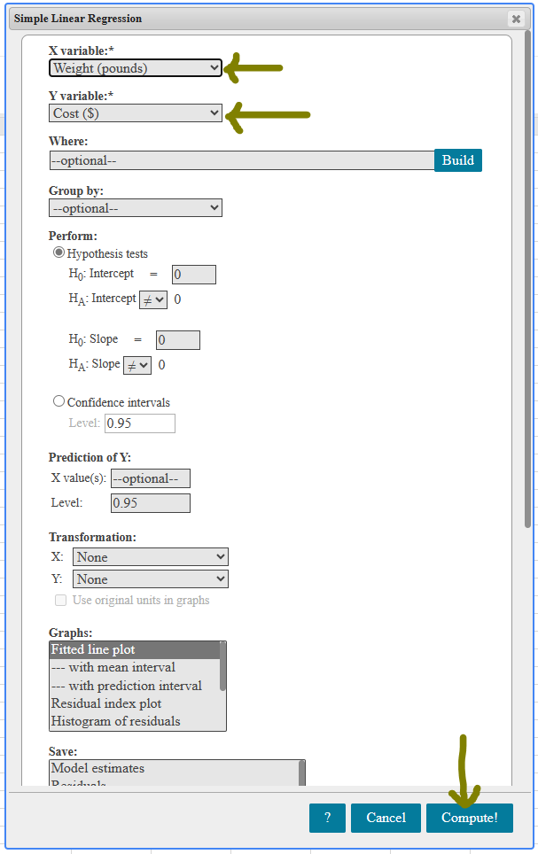
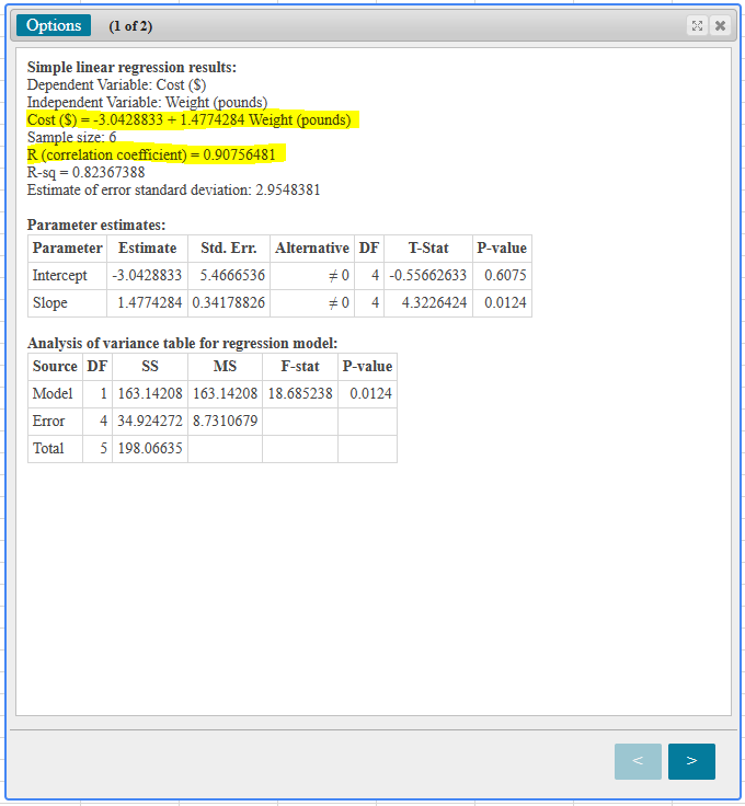
Determine the linear correlation coefficient using technology.
Interpret the linear correlation coefficient.

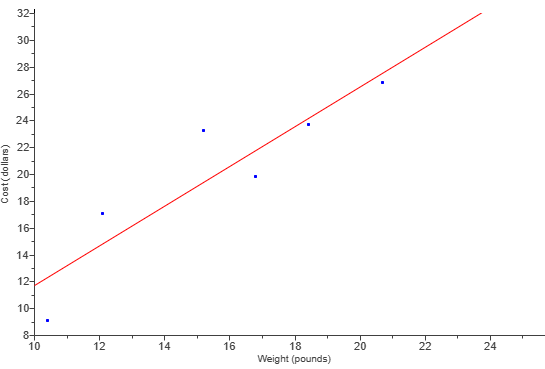
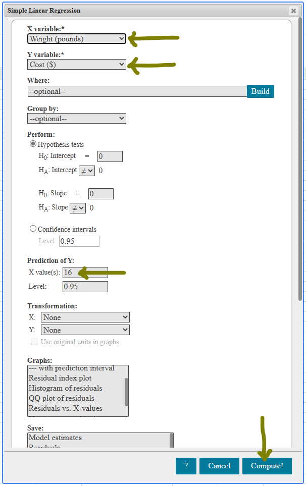
(5.) Linear Regression
Interpret the variables in the linear regression equation.

(I.) Positive Linear Correlation and Negative Linear Correlation:
(a.) Write the least-squares regression line.
(b.) Predict the value of the response variable, given an applicable value of the predictor variable.

(II.) No Linear Correlation:
Because the linear regression equation is used for predictions only if the linear correlation coefficient indicates a linear correlation between the two variables, determine the best value for the response variable given an applicable value of the predictor variable.

NOTE: Do not use any dataset that has a perfectly linear positive linear correlation (r = 1) or a perfectly negative linear correlation (r = −1)
This is because it defeats the purpose of the project.
The project is not designed for you to use the Slope-Intercept form of the equation of a straight line $y = mx + b$
It is designed for you to use the Least-Squares regression line (which is also written in slope-intercept form).

(6.) Sample Size
At least a sample size of 5 (n ≥ 5) is required for each application.

(7.) This is an individual project.
You may collaborate with one another. However, it is not a group project.
No two students should use the same dataset and same variable(s) because there are many datasets available for you.
Be it as it may, I am here to help you. You have my number. Feel free to text me anytime. We can arrange Zoom sessions so I share my screen and work you through any questions you have. Please do this as soon as possible. Keep the due dates in mind.

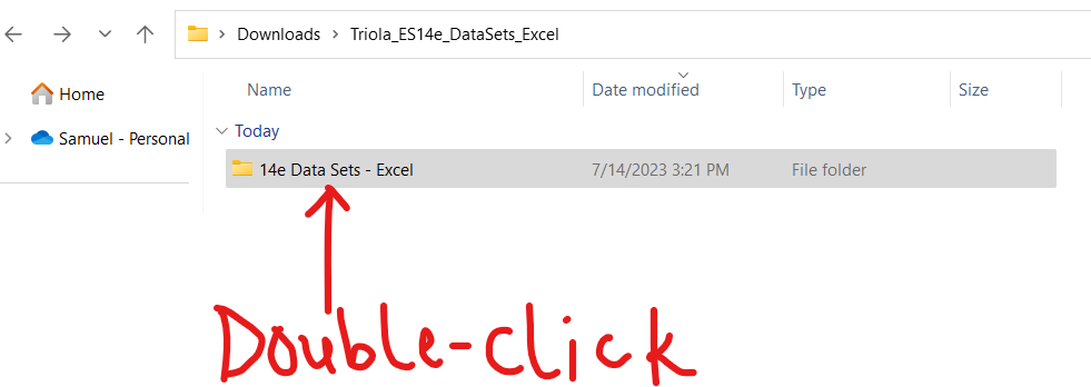
(a.) Please submit the two datasets (names of the datasets including the sources) that you intend to work on, in the Projects: Datasets forum in the Canvas course. I shall review and respond.

(b.) Once I give you the approval, please send your draft to me via email (if you prefer my review to be seen by you alone) or submit your draft in the Projects: Drafts forum in the Canvas course (if you do not mind your colleagues reading my review). I shall review and respond.

(c.) When everything is fine (after you make changes as applicable based on my feedback), please submit your work in the appropriate area (Assignments: Projects page) of the Canvas course.
Only projects submitted in the appropriate area of the Canvas course are graded.
Draft projects are not graded. In other words, projects submitted via email and/or in the Projects: Drafts forum are not graded because they are drafts.
Submitting drafts is highly recommended. If your professor gives you an opportunity to submit a draft, please use that opportunity.
Submitting drafts is not required. It is highly recommended because I want to give you the opportunity to do your project very well and make an excellent grade in it.

(8.) As a student, you have free access to Microsoft Office suite of apps.
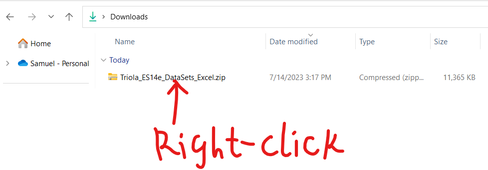
(a.) Please download the desktop apps of Microsoft Office on your desktop/laptop (Windows and/or Mac only).
Do not use a chromebook. Do not use a tablet/iPad. Do not use a smartphone.
Do not use the web app/sharepoint access of Microsoft Office.
(Please contact the IT/Tech Support for assistance if you do not know how to download the desktop app.)
In that regard, the project is to be typed using the desktop version/app of Microsoft Office Word only.

(b.) The file name for the Microsoft Office Word project should be saved as: firstName–lastName–project
Use only hyphens between your first name and your last name; and between your last name and the word, project.
No spaces.

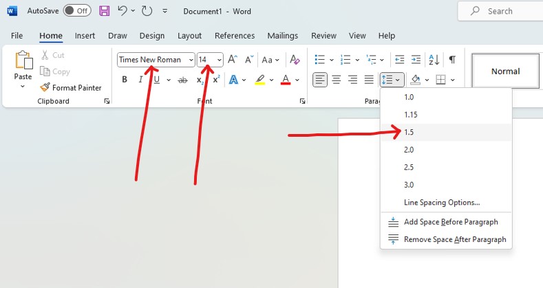
(c.) For all English terms (entire project): use Times New Roman; font size of 14; line spacing of 1.5


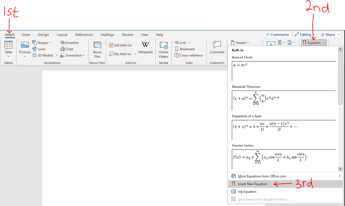
(d.) For all Math terms: symbols, variables, numbers, formulas, expressions, equations and fractions among others, please use the Math Equation Editor.
(i.) Set the font to Cambria Math; font size of 14; and align accordingly
(ii.) Insert a space after each each equation as applicable. Just make a good work that is organized and spacious.
(iii.) Align the functions in each piece of the piecewise function accordingly.







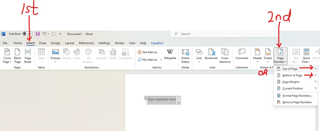
(e.) Include page numbers. You may include at the top of the pages or at the bottom of the pages but not both.


(9.) All work must be shown.
Please write each formula before you use it.
If you use any variables, please define your variables accordingly in the context of your application.

(10.) All work must be turned in by the final due date to receive credit.
It is highly recommended that you turn in your draft by the first due date.
Then, review my feedback and make corrections as necessary and keep working with me until I give you the green light to turn it in.
This must be done by the final due date.
I would not wait till the due dates: the sooner you turn it in, the better.

Example Guides (Correlation and Regression Project)

Symbols

Formulas

$ (1.)\;\; \bar{x} = \dfrac{\Sigma x}{n} \\[5ex] (2.)\;\; \bar{y} = \dfrac{\Sigma y}{n} \\[5ex] (3.)\;\; z_{x} = \dfrac{x - \bar{x}}{s_{x}} \\[5ex] (4.)\;\; z_{y} = \dfrac{y - \bar{y}}{s_{y}} \\[5ex] $ First Formula for Standard Deviation

$ (5.)\;\; s_{x} = \sqrt{\dfrac{\Sigma(x - \bar{x})^2}{n - 1}} \\[7ex] (6.)\;\; s_{y} = \sqrt{\dfrac{\Sigma(y - \bar{y})^2}{n - 1}} \\[7ex] $ Second Formula for Standard Deviation

$ (7.)\;\; s_{x} = \sqrt{\dfrac{n(\Sigma x^2) - (\Sigma x)^2}{n(n - 1)}} \\[7ex] (8.)\;\; s_{y} = \sqrt{\dfrac{n(\Sigma y^2) - (\Sigma y)^2}{n(n - 1)}} \\[7ex] $ First Formula for Pearson Correlation Coefficient

$ (9.)\;\; r = \dfrac{\Sigma\left(\dfrac{x - \bar{x}}{s_x}\right)\left(\dfrac{y - \bar{y}}{s_y}\right)}{n - 1} \\[7ex] (10.)\;\; r = \dfrac{\Sigma\left(z_x\right)\left(z_y\right)}{n - 1} \\[5ex] $ Second Formula for Pearson Correlation Coefficient

$ (11.)\;\; r = \dfrac{n(\Sigma xy) - (\Sigma x)(\Sigma y)}{\sqrt{n(\Sigma x^2) - (\Sigma x)^2} * \sqrt{n(\Sigma y^2) - (\Sigma y)^2}} \\[7ex] $ Slope of the Least-Squares Regression Line

$ (12.)\;\; b_1 = r * \dfrac{s_y}{s_x} \\[7ex] $ Y-intercept of the Least-Squares Regression Line

$ (13.)\;\; b_0 = \bar{y} - b_1 * \bar{x} \\[3ex] $ Least-Squares Regression Line
or
Line of Best Fit
or
Linear Regression Equation

$ (14.)\;\; \hat{y} = b_{1}x + b_0 \\[3ex] $

Critical Values for Pearson's Linear Correlation Coefficient

Unless stated otherwise:
(1.) Use α = 5% = 0.05 (Proportion in TWO Tails)
(2.) df = n − 2
(3.) n = df + 2

Set up the Texas Instruments (TI) Calculator

The first thing we need to do is to turn Diagonstic On

(1.)

(2.)

(3.)

Positive Linear Correlation: Scatter Diagram, Correlation Coefficient, Linear Regression

Dataset: turkeys
Source: MyLab Math
Description:
The table shows a list of the weights and costs of some turkeys at different supermarkets.



Does the cost of turkey depend on the weight, or does the weight of turkey depend on the cost?
X = Independent Variable: Weight (pounds)
Y = Dependent Variable: Cost ($)

Scatter Diagram using Pearson Statcrunch








Correlation Coefficient by Formulas
First Formula will be used for this example

$ r = \dfrac{\Sigma\left(\dfrac{x - \bar{x}}{s_x}\right)\left(\dfrac{y - \bar{y}}{s_y}\right)}{n - 1} \\[5ex] $ Simplify it with the TI Calculator


Enter in the data for the x-values and the y-values



Calculate the mean for the X-variable and the Y-variable

$ L_1 = x \\[3ex] L_2 = x - \bar{x} \\[3ex] \bar{x} = \dfrac{\Sigma x}{n} \\[5ex] \bar{x} = \dfrac{93.6}{6} \\[5ex] \bar{x} = 15.6 \\[5ex] \bar{y} = \dfrac{\Sigma y}{n} \\[5ex] \bar{y} = \dfrac{120.03}{6} \\[5ex] \bar{y} = 20.005 \\[3ex] $ Calculate the standard deviation for the X-variable and the Y-variable
Write the formulas for the first set of lists accordingly
Each list is automatically populated after writing the formula
For example:

$ L_3 = x - \bar{x} = L_1 - 15.6 \\[4ex] $



$ L_4 = (x - \bar{x})^2 = L_3^2 \\[4ex] L_5 = y - \bar{y} = L_2 - 20.005 \\[4ex] L_6 = (y - \bar{y})^2 = L_5^2 \\[4ex] $

Let us write what we have so far.
Let us also calculate the standard deviation.

$x$	$x - \bar{x}$	$(x - \bar{x})^2$	$y$	$y - \bar{y}$	$(y - \bar{y})^2$
12.1	−3.5	12.25	17.13	−2.875	8.265625
18.4	2.8	7.84	23.75	3.745	14.025025
20.7	5.1	26.01	26.86	6.855	46.991025
16.8	1.2	1.44	19.83	−0.175	0.030625
15.2	−0.4	0.16	23.31	3.305	10.923025
10.4	−5.2	27.04	9.15	−10.855	117.831025
$ \Sigma (x - \bar{x})^2 = 74.74 \\[3ex] n - 1 = 6 - 1 = 5 \\[3ex] s_{x} = \sqrt{\dfrac{\Sigma(x - \bar{x})^2}{n - 1}} \\[5ex] s_x = \sqrt{\dfrac{74.74}{5}} \\[5ex] s_x = \sqrt{14.948} \\[3ex] s_x = 3.866264347 $			$ \Sigma (y - \bar{y})^2 = 74.74 \\[3ex] n - 1 = 6 - 1 = 5 \\[3ex] s_{y} = \sqrt{\dfrac{\Sigma(y - \bar{y})^2}{n - 1}} \\[5ex] s_y = \sqrt{\dfrac{198.06635}{5}} \\[5ex] s_y = \sqrt{39.61327} \\[3ex] s_y = 6.293907371 $

Verify the Mean and Standard Deviation using TI-series calculator








Write the formulas for the second set of lists accordingly
Each list is automatically populated after writing the formula

$ L_1 = x - \bar{x} \\[3ex] L_2 = \dfrac{L_1}{s_x} = \dfrac{L_1}{3.866264347} \\[5ex] L_3 = y - \bar{y} \\[3ex] L_4 = \dfrac{L_2}{s_y} = \dfrac{L2}{6.293907371} \\[5ex] L_5 = L_2 * L_4 \\[3ex] $

$x - \bar{x}$	$\dfrac{x - \bar{x}}{s_x}$	$y - \bar{y}$	$\dfrac{y - \bar{y}}{s_y}$	$\left(\dfrac{x - \bar{x}}{s_x}\right)\left(\dfrac{y - \bar{y}}{s_y}\right)$
−3.5	−0.905266605	−2.875	−0.456790961	0.4135176030
2.8	0.724213284	3.745	0.595019878	0.430921300
5.1	1.31910276	6.855	1.08914853	1.43669884
1.2	0.310377121	−0.175	−0.02780466	−0.00862993
−0.4	−0.10345904	3.305	0.525111001	−0.05432748
−5.2	−1.3449675	−10.855	−1.7246837	2.31964368
				$ \Sigma\left(\dfrac{x - \bar{x}}{s_x}\right)\left(\dfrac{y - \bar{y}}{s_y}\right) = 4.537824013 \\[7ex] n - 1 = 5 \\[5ex] r = \dfrac{\Sigma\left(\dfrac{x - \bar{x}}{s_x}\right)\left(\dfrac{y - \bar{y}}{s_y}\right)}{n - 1} \\[7ex] r = \dfrac{4.537824013}{5} \\[5ex] r = 0.9075648026 $

Type of Linear Relationship

$ Calculated\;\;value\;\;of\;\;r = 0.9075648026 \\[3ex] |r| = |0.9075648026| = 0.9075648026 \\[5ex] n = 6 \\[3ex] df = 6 - 2 = 4 \\[3ex] Critical\;\;value\;\;of\;\;r = 0.8114 \\[5ex] 0.9075648026 \gt 0.8114 \\[3ex] $ Because the absolute value of the calculated value of the correlation coefficient is greater than the critical value of the correlation coefficient, there is a positive linear correlation between the costs of the turkeys and the weights of the turkeys.
We shall now calculate the linear regression equation so we can use it for prediction of a cost, given a weight.

Linear Regression Equation using TI-series calculator








Linear Regression Equation using Formulas

$ b_1 = r * \dfrac{s_y}{s_x} \\[5ex] b_1 = 0.9075648026 * \dfrac{6.293907371}{3.866264347} \\[5ex] b_1 = 1.477428414 \\[5ex] b_0 = \bar{y} - b_1 * \bar{x} \\[3ex] b_0 = 20.005 - 1.477428414(15.6) \\[3ex] b_0 = -3.042883252 \\[5ex] \underline{Line\;\;of\;\;Best\;\;Fit} \\[3ex] \hat{y} = b_1x + b_0 \\[3ex] \hat{y} = 1.477428414x + -3.042883252 \\[3ex] \hat{y} = 1.477428414x - 3.042883252 \\[3ex] $ Interpretation of the Slope and Y-Intercept of the Linear Regression Equation
Slope = 1.477428414
Slope ≈ $1.48
This implies that for each increase of 1 pound in the weight of the turkey, the cost increases by an average of approximately $1.48

Y-intercept = −3.042883252
Y-intercept approx −$3.04
The interpretation of the Y-intercept is not appropriate because:
(1.) It is not possible to have a turkey that weighs 0 pounds
(2.) The cost of 0 pounds of turkey cannot be a negative value.

Interpretation of the Coefficient of Determination
r² = 0.8236738762
r² = 82.36738762%
This implies that 82.36738762% of the variation in cost is explained by the weight of the turkeys.

Prediction using the Linear Regression Equation
Minimum weight = 10.4 pounds
Maximum weight = 20.7 pounds
Predict the cost for a weight of 16 pounds

$ \hat{y} = 1.477428414x - 3.042883252 \\[3ex] x = 16\;pounds \\[3ex] \hat{y} = 1.477428414(16) - 3.042883252 \\[3ex] \hat{y} = 20.59597137 \\[3ex] \hat{y} \approx \$20.60 \\[3ex] $ The cost of a turkey that weighs 16 pounds is approximately $20.60

Linear Regression Equation and Correlation Coefficient using Pearson Statcrunch






Line of Best Fit in Scatter Diagram using Pearson Statcrunch


Prediction using Pearson Statcrunch
Minimum weight = 10.4 pounds
Maximum weight = 20.7 pounds
Predict the cost for a weight of 16 pounds

Prediction using Statcrunch




The cost of a turkey that weighs 16 pounds is approximately $20.60

Negative Linear Correlation: Scatter Diagram, Correlation Coefficient, Linear Regression

Dataset:
Source:
Description:




Does the ... depend on the ..., or does the ... depend on the ...?
Independent Variable:
Dependent Variable:

Scatter Diagram using Pearson Statcrunch

No Linear Correlation: Scatter Diagram, Correlation Coefficient

Dataset:
Source:
Description:




Does the ... depend on the ..., or does the ... depend on the ...?
Independent Variable:
Dependent Variable:

Scatter Diagram using Pearson Statcrunch

Students Projects

References

Chukwuemeka, Samuel Dominic (2023). R and RStudio Statistics Software. Retrieved from https://statistical-science.appspot.com/

Sullivan, M., & Barnett, R. (2013). Statistics: Informed decisions using data with an introduction to mathematics of finance (2nd custom ed.). Boston: Pearson Learning Solutions.

Triola, M. F. (2015). Elementary Statistics using the TI-83/84 Plus Calculator (5th ed.). Boston: Pearson

Triola, M. F. (2022). Elementary Statistics. (14th ed.) Hoboken: Pearson.

Critical Values for Pearson’s Correlation Coefficient. (n.d.). http://commres.net/wiki/_media/correlationtable.pdf